Data Quality Is Not a Property of Data
Published:
TL;DR: Data quality is not a property of the data. It is the marginal value of a sample relative to the model, the training stage, and the data already seen. The mixture tables we tune today are mostly a side-effect of how the data happened to be stored.
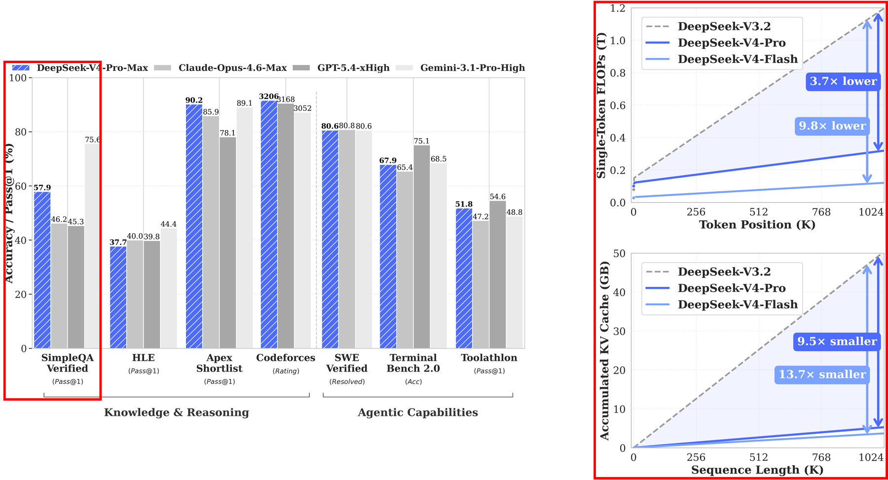 Figure 1: Header figure (Figure 1) of the DeepSeek-V4 technical report. Left: a knowledge benchmark. Right: long-context efficiency. Used here as a hook, not as evidence for any data-mixture claim.
A small model’s parameter count, training tokens, and knowledge capability do not form a simple ordering. DeepSeek puts SimpleQA-Verified on the front of its V4 report; on hard-knowledge leaderboards like AA-Omniscience — which scale almost monotonically with model size — small models still beat a long list of much larger ones (see Figure 2). These two observations are where this inquiry starts, not proof of any conclusion.
The lens of this post: data quality is not a static property of a sample. It is the marginal value of that sample relative to the model, the training stage, and the data already seen.
1. The inherited taxonomy
The Pile’s 22 components — CommonCrawl, GitHub, arXiv, Books, Wikipedia, StackExchange … — are fundamentally a collection manifest: which crawler, which API the data was pulled from. Yet the field has since treated it as a semantic taxonomy, and spent years doing mixture search on top of it, producing tables like “X% code, Y% web.”
Provenance is the purest expression of the “data has properties” mindset: it is a static label stamped onto a sample at the moment of collection, before any model saw it. The whole taxonomy is built on mistaking that stamp — where the data came from — for what the data is. Mixture search reweights by provenance not because provenance is the right semantic axis, but because it happens to supply the cheapest, most stable, most operable bucketing key we have: cost, licensing, traceability, and contamination control all ride on it. That is a deeper explanation than “we were lazy,” and it is why the taxonomy persists.
One check: open any recent data-mixture paper, and its axes are almost always data sources, not semantic categories. The point is not that anyone can verify it in five seconds; it is that the search space was inherited from the storage system, not derived from a learning problem.
2. A known objective the pipeline never adopted
Deduplication and a quality classifier are often described as if they rest on “contradictory assumptions.” That framing is too clean. A pointwise quality classifier does not assume total value is additive; it only uses a pointwise proxy at one stage. Deduplication does not assume value is non-additive; it estimates the interaction between samples. The real, less tidy observation is that a single pipeline deploys two value approximations at different levels, yet rarely calibrates the two together:
where q(xi) is the pointwise quality of a sample and s(xi, xj) is its redundancy with others. Quality asks “is this document good on its own?”; dedup asks “given the other documents, is it still worth keeping?” A pipeline needs both questions, yet typically gives only the first one an explicit score — and almost never models how the two jointly determine a sample’s marginal value.
Worth stating plainly: this joint objective is not unwritten. Combining a per-sample quality term with a redundancy-interaction term reflects an idea that has appeared separately in submodular selection, DPP, and MMR: jointly considering quality, coverage, and redundancy — and data subset selection has a whole line of work built on it. So “the two approximations were never reconciled” overstates it: what is studied is not missing; what is missing is its unified adoption in production pipelines. The gap is between theory and engineering, not a void in knowledge.
3. “Optimal mixture” is an ill-posed question
Most technical reports still present the mixture as a static percentage table, even when the actual training uses a staged data schedule. Annealing and mid-training reweighting — Llama 3’s annealing stage, OLMo 2’s Dolmino mid-training mix — are open practice. The notation hides the time axis: a mixture is not a point but a schedule. So the very question “what is the optimal mixture” is ill-posed until you specify when in training you mean. This is a complete, verifiable observation in its own right, and it is one more reason the static tables from §1 are a residue of the storage system, not a description of the real optimization.
4. Why the problem stayed invisible
4.1 Importance and visibility are diverging
Of the swarm of attention variants from 2018–2022, very few survived into production; yet under the same architecture family, models from different labs diverge sharply in their knowledge profiles. Read any recent technical report: the architecture section is illustrated down to the hyperparameters, while the data section is often a single sentence — “high-quality, diverse, multi-source.” What is striking is not that data is under-disclosed, but that the importance of data methods and their observability are moving in opposite directions.
A reproducibility view of the same reports makes the pattern cleaner than a word count (word count conflates how much was said with how much was disclosed — a closed lab can write 3.9k words and say nothing):
| Report | Architecture reproducible? | Corpus composition reproducible? |
|---|---|---|
| OLMo 2 (2024) | yes | yes |
| Llama 3 (2024) | yes | partial |
| DeepSeek-V4 (2026) | partial | partial |
| Mistral 7B (2023) | yes | no |
| Mixtral 8x7B (2024) | yes | no |
| Frontier closed models | no report | no report |
The interesting rows are the ones where architecture is reproducible but the corpus is not (Mistral, Mixtral). And the frontier models that publish no report at all are the natural footnote: the more a lab treats its data as the source of value, the less it discloses — so the very models where data matters most are exactly the ones we cannot inspect.
4.2 The hill-climbability bias among benchmarks
Among the headline benchmarks of 2024–2026, the post-training-movable ones (AIME, SWE-bench, GPQA, ARC-AGI) vastly outnumber the post-training-resistant ones (SimpleQA and various knowledge probes). SimpleQA’s marginalization is not a matter of taste; it is a hill-climbability bias in the benchmark ecosystem: evaluations that current methods can keep pushing — and that keep separating the leading models — are the ones that stay center stage.
Why are knowledge probes “resistant”? Not because post-training is powerless, but because it mostly cannot create underlying factual coverage — it can change extraction, refusal, and calibration, not the store of facts a model absorbed at pre-training. These methods treat factual capacity as a relatively stable quantity after pre-training; this supports the claim that post-training can hardly create underlying factual coverage — but it does not mean evaluation scores cannot shift through extraction, refusal, and calibration. SimpleQA-Verified (Haas et al., 2025) is the careful, low-label-noise version of that factual benchmark. So the “post-training can hardly create underlying factual coverage” half has a basis.
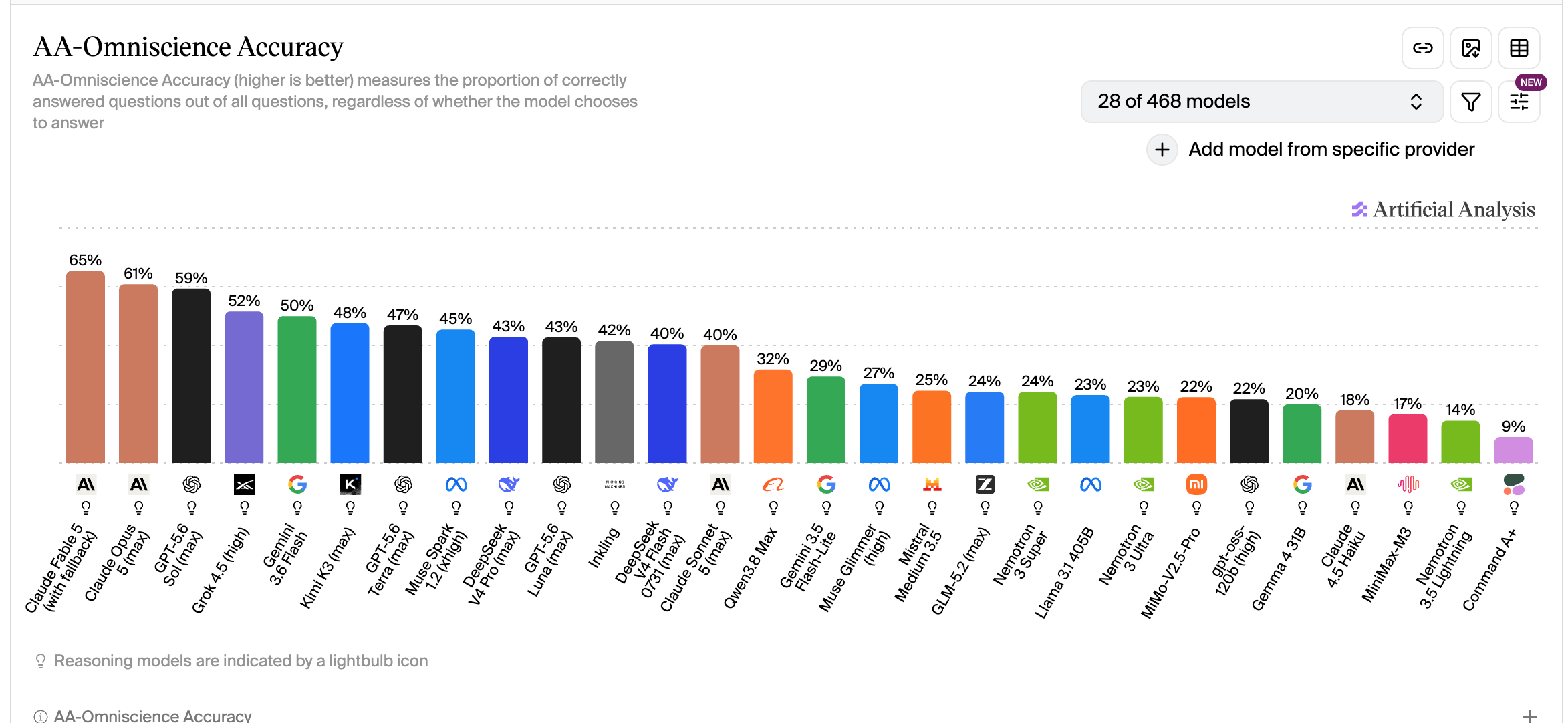 Figure 2: AA-Omniscience Accuracy cross-model leaderboard (top 28). Hard-knowledge leaderboards like this are among the few windows post-training struggles to move — the starting point for the argument above.
5. The experiment this perspective calls for
Sections 4.1 and 4.2 together explain why the puzzle from §4.1 — same architecture family, sharply different knowledge profiles across labs — has never been cleanly attributed to data. To attribute it cleanly, you would run a controlled comparison whose treatment and control do not overlap:
- Same candidate pool, same architecture and optimizer, same token budget, same post-training, same random seeds for repeated runs: these are the real inputs to training, and should be held fixed.
- The only thing that varies is the sampling weight: this is the single handle you turn — the allocation across domains, not the volume.
- Report, rather than pre-control, real coverage: dedup strength, the actual observed unique-token coverage, per-domain exposure and duplicate-exposure rate should be measured and reported as observables — not locked down in advance, or you may also control away the very mechanism by which the mixture acts.
- Eval: use factual / knowledge benchmarks (whose factual coverage is relatively stable after pre-training, e.g. SimpleQA-Verified or Incompressible Knowledge Probes) to measure the factual-capacity gap caused by the allocation.
If you want to measure dedup strength on its own, that is a second, independent experiment and should not be bundled into the same design.
The prediction is falsifiable: if allocation (not volume) is the driver, then after matching the actually observed unique-token coverage and per-domain exposure, the knowledge-profile gap should persist; if the gap disappears once coverage is matched, then the driver is volume, not allocation. One honest caveat: a single pair (n = 2) cannot separate “the recipe” from “this one recipe” — strictly you want a small sweep over allocation weights, not one contrast.
But among public experiments, I have not yet seen one that satisfies all of the above at once: DoReMi, RegMix, DCLM, DataComp-LM, and a large body of data-selection ablations have run experiments that fix the model and budget and vary the data strategy, yet few use factual-capacity probes to measure knowledge coverage specifically, and they usually do not fix post-training. The question most worth answering cleanly falls into the blind spot of “neither visible nor specifically tested” — the existing public evidence is not yet sufficient to answer it.
6. Why every technique is only a proxy
Semantic deduplication (see the semantic-deduplication layer described in MAI-Thinking-1, Microsoft AI, 2026), domain mixture, quality filtering, loss-based sampling, curriculum learning — they are not the same technique, but they are all approximations of the same target: where the next unit of training budget for different data should go. Saying they “are really the same thing” overstates it, but they share a narrower, truer claim: each is a different proxy for marginal value, and none of them is the quantity itself.
The reason is not in the implementation; it is in measurability. These five proxies are proxies because they are measurable, while the target is not. Marginal value can only be measured by a counterfactual training run — train more on this class of data, what does the model actually gain? What can be directly optimized is the proxy; what cannot is the target — and the target is, by definition, a counterfactual.
7. The counterfactual is the point
That counterfactual — not any bucket schedule — is the operational form of the thesis. It is also what makes density×diversity frameworks (Chen et al., ACL 2025, Figure 3) seductive and dangerous at once: sorting data into buckets by density × diversity and assigning each a sampling rate sounds like an executable target. But “rare, hard-to-learn data deserves more weight” is neither a proven universal law nor safe as one — rarity can mean worthlessness, difficulty can mean noise, and boosting noise mistaken for valuable long-tail is worse than ignoring the tail. Reliability and relevance-to-target constraints have to be added separately, on top of the framework.
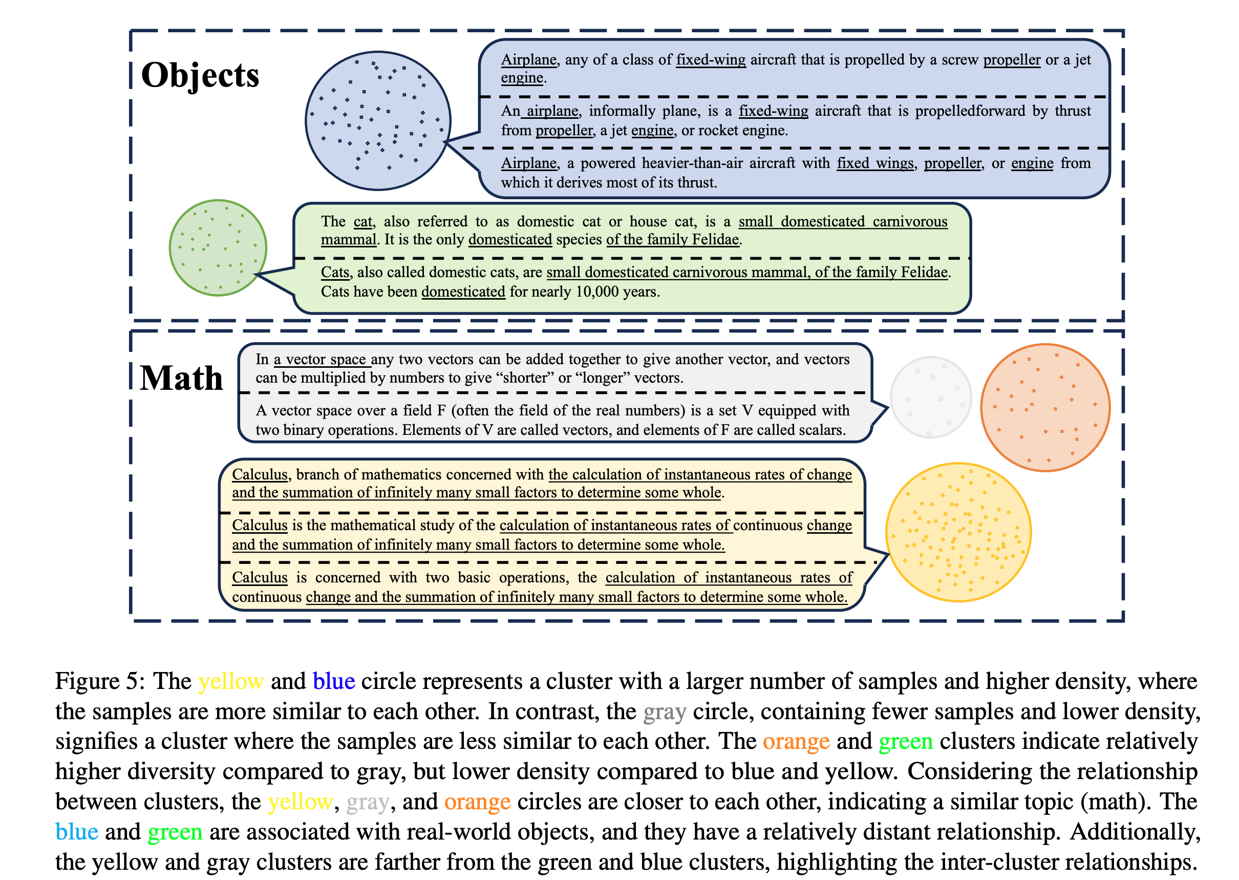 Figure 3: Chen et al., ACL 2025, Figure 5. Within one corpus, clusters split along density (how packed the points are) and diversity (how similar the points are).
8. Closing
The taxonomy we inherited (§1), the hill-climbability bias among benchmarks (§4.2), and the experiment this perspective calls for (§5) — they all point at one thing: a datum’s value is not a property of the datum, but its marginal value relative to the model, the training stage, and the data already seen.
The next phase of data engineering may stop asking “is this datum good” and start asking “given what the model has already seen, where is the next token budget best spent.” That is a framework, not a recipe; this post does not answer it, only makes it legible.
References
- Bojie Li. Incompressible Knowledge Probes: Estimating Black-Box LLM Parameter Counts via Factual Capacity. Pine AI, 2026. arXiv:2604.24827.
- Lukas Haas, Gal Yona, Giovanni D’Antonio, Sasha Goldshtein, Dipanjan Das. SimpleQA Verified: A Reliable Factuality Benchmark to Measure Parametric Knowledge. Google DeepMind / Google Research, 2025. arXiv:2509.07968.
- Meta AI. The Llama 3 Herd of Models. 2024. arXiv:2407.21783.
- Team OLMo, Pete Walsh, Luca Soldaini, et al. OLMo 2: The Best Way to Train Open Language Models. AI2, 2024. arXiv:2501.00656.- Alex Kulesza and Ben Taskar. Determinantal Point Processes for Machine Learning. Foundations and Trends in Machine Learning, 2012.
- Microsoft AI. MAI-Thinking-1: Building a Hill-Climbing Machine. Microsoft, 2026.
- DeepSeek-AI. DeepSeek-V4: Towards Highly Efficient Million-Token Context Intelligence. 2026. arXiv:2606.19348.
- Artificial Analysis. Omniscience Evaluations. artificialanalysis.ai/evaluations/omniscience.
- Zhengyu Chen, Siqi Wang, Teng Xiao, Yudong Wang, Shiqi Chen, Xunliang Cai, Junxian He, Jingang Wang. Revisiting Scaling Laws for Language Models: The Role of Data Quality and Training Strategies. ACL 2025. Link.
- Gao et al. The Pile: An 800GB Dataset of Diverse Text for Language Modeling. 2020. arXiv:2101.00027.